Structural risk minimization

I have been studying the model selection problem during the past few months and this is a personal study note.

The structural risk minimization (SRM) is an important method for model selection in statistical learning. The choice of the hypothesis function model is nontrivial since there exists a trade-off concerning the model complexity. Considering a classification task, the ideal classifier is less likely to contain in a simplistic model, while learning a complex model consumes substantial computation and risks overfitting.

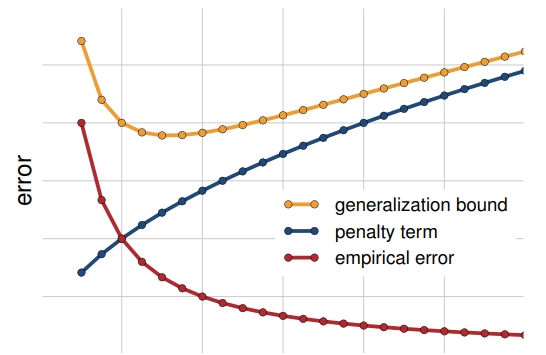
SRM balances the estimation error and approximation error of the learning through minimizing the sum of empirical risk and penalty term for model complexity. As the model becomes rich and complex, the empirical risk decreases and changes little while the penalty term goes larger.

Empirical risk

Empirical risk minimization is to minimize the estimation error on the given training data $\mathcal{T}$.

Rademacher complexity

Rademacher complexity measures the capacity of a hypothesis class of real-valued functions. Denote $\mathcal{X}, \mathcal{Y}$ as the input and output spaces in a regression problem. $\mathcal{F}$ is a hypothesis function class, where $f:\mathcal{X} \xrightarrow{} \mathcal{Y}, f\in \mathcal{F}$. For an arbitrary loss function class $\mathcal{L}$ associated with $\mathcal{F}$ mapping from $\mathcal{Z} = \mathcal{X} \times \mathcal{Y}$ to $\mathbb{R}$, we have

We then provide the following definition.

Definition 1 Given $\mathcal{L}$ as a function class mapping from $\mathcal{Z}$ to $\mathbb{R}$, and $S=\{z_i\}_{i=1}^m$ as a sequence of $m$ samples from $\mathcal{Z}$, the empirical Rademacher complexity of $\mathcal{L}$ with respect to $S$ is defined as

\[\hat{\mathfrak{R}}_S(\mathcal{L}) = \mathbb{E}_{\sigma} \left[ \sup_{l\in \mathcal{L}} \frac{1}{m} \sum_{i=1}^m \sigma_i l(z_i) \right],\]

where $\sigma = (\sigma_i)_{i=1}^m$ are independent uniform random variables distributed in ${-1,1}$. $\sigma_i$ is called Rademacher variable. The Rademacher complexity of $\mathcal{L} $ is $\mathfrak{R}_m(\mathcal{L} ) = \mathbb{E}_{S} \hat{\mathfrak{R}}_S(\mathcal{L})$.

The Rademacher complexity provides an upper bound on the difference between the empirical risk and the expected risk. The generalization bound is presented as follows.

Theorem 1 (One-sided bound) Let $\mathcal{L} $ be a function class mapping from $\mathcal{Z}$ to $[a,b]$ and $S=\{z_i\}_{i=1}^m$ be a sequence of $m$ i.i.d. samples from $\mathcal{Z}$. Then for any $\delta>0$, with at least $1-\delta$ probability

\[\mathbb{E}[l (z)] -\frac{1}{m} \sum_{i=1}^m l (z_i) \leq 2 \hat{\mathfrak{R}}_S(\mathcal{L} ) + 3 (b-a) \sqrt{\frac{\log \frac{2}{\delta}}{2m}}\]

holds for all $l \in \mathcal{L}$.

(Two-sided bound) For any $\delta>0$, with at least $1-\delta$ probability

\[\sup_{l \in \mathcal{L} } \left|\mathbb{E}[l (z)] - \frac{1}{m} \sum_{i=1}^m l (z_i) \right| \leqslant 2 \hat{\mathfrak{R}}_S(\mathcal{L} ) + 3 (b-a) \sqrt{\frac{\log \frac{4}{\delta}}{2m}}\]

The Rademacher complexity possesses some important properties, which are helpful in calculation.

• If $F \subseteq H$, then $\mathfrak{R}_m(F) \leq \mathfrak{R}_m(H)$.
• for any $c\in \mathbb{R}$, $\mathfrak{R}_m(cF)=|c|\mathfrak{R}_m(F)$.
• if $l:\mathbb{R} \rightarrow \mathbb{R}$ is Lipschitz with constant $L$ and satisfies $l(0)=0$, then $\mathfrak{R}_m(l(F)) \leq 2L\mathfrak{R}_m(F)$.
• $\mathfrak{R}_m(F) = \mathfrak{R}_m(\mathrm{conv}F)$.
• $\mathfrak{R}_m (\sum_{k=1}^C F_k) \leq \sum_{k=1}^C \mathfrak{R}_m(F_k)$.

Structural risk

SRM consists of selecting an optimal reward function class index $1 \leq k^* \leq C$ and the ERM hypothesis $f^* \in \mathcal{F}_{k^*}$ which minimizes both estimation error and the model complexity penalty.

Since we cannot obtain the real value of $\mathfrak{R}_m(F_k)$, substitute with the empirical Rademacher complexity $\hat{\mathfrak{R}}_m(F_k)$. As for why we multiply $2$ here for $\mathfrak{R}_m(F_k)$, one reason is for the subsequent theorem derivation (in order to utilize Theorem 1). It is natural to do a weighted up between empirical risk and model penalty, while I have not figured out how to guarantee the learning bound in such instance.

Theorem 2 (SRM learning guarantee) For the SRM solution $f^{SRM}_{\mathcal{T}}$, with the probability $1-\delta$

\[\epsilon_{\mathcal{D}}(f_{\mathcal{T}}^{SRM}) \leqslant \inf_{f \in \mathcal{F}} \left( \epsilon_{\mathcal{D}}(f) + 4 \mathfrak{R}_m({\mathcal{F}}_{k(f)}) \right)+ 3 (b-a) \sqrt{\frac{\log \frac{4(C+1)}{\delta}}{2m}}\]

holds.